
Frequency tables and Frequency Distributions
Introduction
Before preparing frequency distribution it is necessary to collect data of the required nature from the various sources. The data collected is always in raw form which is needed to be arranged in a proper arrangement for the purpose of inferring the required results. You need to do certain preparations for frequency distribution, which includes the classification and tabulation of data. Both of them are explained in detail as follows;
Classification
“The process of arranging data into classes or categories according to some common characteristics present in the data is called classification”
Collected data are usually available in a form which is not easy to comprehend. For example, if we have before us the marks obtained by 1000 universities students at their Undergraduate Examination, it would be difficult to tell simply by looking at the marks as to how many students have marks between 300 and 400, between 400 and 500, and so on. In order to get the clear picture of the situation, the data must be present in a manner which is easy to understand. As first step, we arrange the data into classes and categories having similar characteristics. For example, we may arrange the marks into groups of 50 marks each, e.g. 300 to 349, 350 to 399, 400 to 449 and so on.
Basis for Classification
The collected data can be classified by many characteristics, there are four main basis of classification are mostly being practiced. These bases are;
1. Qualitative
- When data are classified by attributes, e.g. religion, marital status etc.2.
2. Quantitative:
- When data are classified by quantitative characteristics, e.g. height, weight, income, etc.
3. Geographical:
- When data are classified by geographical regions or locations, e.g. the population of a country may be classified by provinces, divisions, districts or towns.
4. Chronological/Temporal:
When data are classified by their time of occurrence. An arrangement of data by their time of occurrence is called a time series.
Tabulation
“The process of arranging data into rows and columns is called tabulation”
A table is a systematic arrangement of data into vertical column and horizontal rows. Tabulation of data on population of a country can by classified on the basis of religion, gender or marital status. Tabulation may be simple, double, triple or complex depending on the nature of classification, which is being used by the statistician.
Frequency Distribution
“A frequency distribution is a tabular arrangement of data in which various items are arranged into classes and the number of items falling in each class is being mentioned”
We have discussed the classification and tabulation of data. Frequency distribution is an important method of summarizing and organizing quantitative data. The data which is presented in the form of frequency distribution is called grouped data, whereas, the data which has not been arranged in a systematic order or in the form of frequency distribution is called raw data or ungrouped data.
For Example
Let us consider the weight of 120 students at a university, as given below:
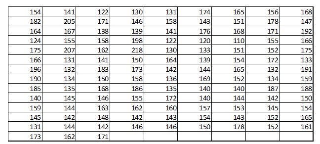
From the above provided data it is difficult to draw any meaningful conclusions. As in, it is difficult to tell simply by looking at the above data as to how many students have weights below or above 150 pounds or between 150 and 200 pounds and so on. Therefore, necessary to arrange the data in such a way as their main features as clear. Conclusion can easily be drawn if the data is arranged in an array. An arrangement of data in ascending or descending order is called an array.
From the array many question regarding the data could be answered. But still it will be difficult to look at 120 observations and obtain an accurate idea as to how these observations are distributed. Therefore, we can arrange them in better form. For example, the data may be arranged into classes as shown in following Table:

By arranging the raw data in the above form we have distributed the data into classes and determined the number of items belonging to each class i.e. class frequency. The range of data from 110 to 119 is a single class and 1 is it’s corresponding frequency. Such an arrangement of data by classes together with their corresponding class frequencies is called frequency distribution or frequency table.
Class Limits
In Table 1 we see that each class is described by two numbers. These numbers are called class limits. The smaller number is called the lower class limit, and the larger number is called upper class limit. For example, in Table 1, the class limits for first class are 110 and 119. 110 is the lower class limit and 119 is the upper class limit.
Class Boundaries
Class limits are not always exactly what they look like. We know that measurements are seldom exact, most of the time they involve approximates and estimations. A weight of 110 pounds means a weight lying between 109.5 and 110.5 pounds. And a weight 119 pounds means a weight lying between 118.5 and 119.5 pounds. When the lower class limit is given as 110 pounds, the true lower class limit is, therefore, the 109.5 pounds and when the upper class limit is given as 119 pounds, the true upper class limit is actually 109.5 pounds. Therefore, if the weights are recorded to the nearest pounds, the class 110–119 includes all the measurements from 109.5 to 119.5 pounds.
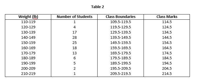
The values 109.5 and 119.5 which describe the true class limits of a class are the called the true class limits or class boundaries. The smaller number 109.5 is lower class boundary and the larger number 119.5 is called upper class boundary. Class boundaries are clearly shown in Table 2.
The class boundary can be obtained by adding the upper class limit of one class to the lower class limit of the next higher class and then dividing by 2. Mathematically it can be represented as following:

For Example, Class boundaries for first class in Table 1 is calculated as:

The following Table 2 shows the class boundaries and class marks for the corresponding classes:
Size of Class Interval
“The size of the class interval, which is also called the class width or class length, is the difference between the upper class boundary and the lower class boundary”.
Class interval is not the difference between the class limits. Where all the class intervals of a frequency distribution are of equal size, the common width id denoted by h. In such case, the size of the class interval is also equal to the difference between the two successive lower or upper class limits. For example, in Table 2 the class interval for first class is 119.5–109.5 = 10, or 120–110 = 10.
Formation of a Frequency Distribution
Following steps are involved in the formation of a frequency distribution:
- Determine the greatest and the smallest number:
First of all determine the greatest and the smallest number in the raw data and find the range, which is the difference between the greatest and the smallest numbers. In the example of weights of 120 students, the greatest number is 218 and the smallest number is 110. Therefore, the range is 218–110 =108.
- Decide on the number of class:
For the purpose of determining the classes for the frequency distribution, there are no hard and fast rules for the purpose. Mostly, 5 to 20 classes are being made. The number of classes should be appropriate, so that could be distributed and represented properly. If we have less than 5 classes, it will result in too much information being lost. On the other hand, if we have more than 20 classes, computation will become unnecessarily lengthy. In Table 1 we have made 11 classes.
- Determine the approximate class interval size:
The approximate class interval size is determined by dividing the range of the desirable number of classes. For example, in the raw data of weights of 120 students, the class interval size is 108/11 = 9.8 or 10. A number used as class interval size should be easy to work with.
- Decide what should be the lower class limit:
The lower class limit should cover the smallest value in the raw data.
- Find the upper-class boundary by adding the class interval size to the lower class boundary:
The upper-class boundary of a particular class is determined by adding the class interval size to the lower class boundary of such class. The remaining lower and upper-class boundaries are determined by adding the class interval repeatedly until the largest measurement of the raw data is enclosed in the final class.
- Distribute the values of the raw data into classes:
The class frequencies are obtained by distributing the raw data measurements into the classes made. The number of measurements falling in each class is referred as it frequency.
Methods for Frequency Distribution
There are two methods for arranging the observations in their proper classes. Such methods are as follows;
- By Listing the Actual Values:
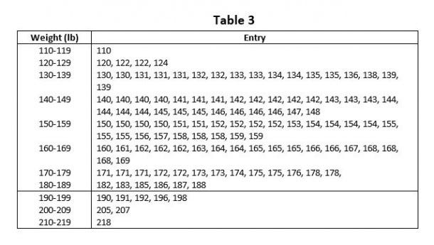
In this method of frequency distribution, each observation is listed in its proper class. The following Table 3 illustrates the tabulation of weight measurements of 120 students. This is called an entry table.
- By Using Tally Marks:
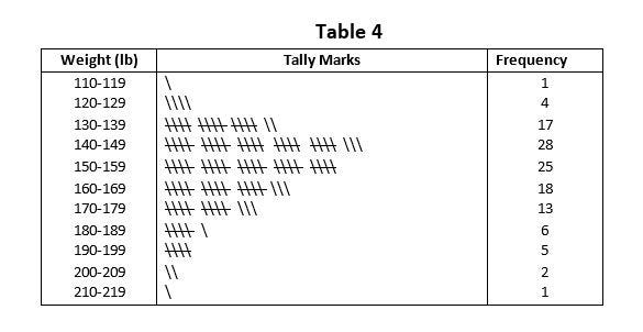
This method of frequency distribution is used where the data are not arranged in order of magnitude. The easiest way of tabulation data is by recording stroke i.e. tally mark, opposite the appropriate class for each observation. The following Table 4 illustrates the frequency distribution by using a tally mark.
Types of Frequency Distribution
- Grouped frequency distribution.
- Ungrouped frequency distribution.
- Cumulative frequency distribution.
- Relative frequency distribution.
- Relative cumulative frequency distribution.
- Bivariate frequency distribution.
Grouped Data
At certain times to ensure that we are making correct and relevant observations from the data set, we may need to group the data into class intervals. This ensures that the frequency distribution best represents the data. Let us make a grouped frequency data table of the same example above of the height of students.
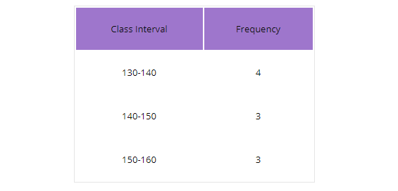
From the above table, you can see that the value of 150 is put in the class interval of 150–160 and not 140–150. This is the convention we must follow. or we can change limits for each class for example 140–149 and 150–159
Frequency Distribution for Discrete Data (Un-Grouped data)
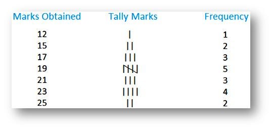
The class limits in discrete data are the true class limits and there will be no class boundaries because discrete data are not in fractions. For example; the following figures represent marks obtained for each student in a certain class.
Cumulative Frequency Distribution
Cumulative frequency distribution represents the sum of all succeeding or previous frequencies up to a certain class. The table showing the cumulative frequency is called cumulative frequency distribution or cumulative frequency distribution table or simply cumulative frequency. For example, referring Table 1, the cumulative frequency for class 120–129 is 1 + 4 = 5. Similarly, the cumulative frequency of the class 130–139 is 1+ 4 + 17 = 22. It will be interpreted as there are 22 children who have weights less than 139.5 pounds. The cumulative frequency is shown in the following table:

Relative Frequency Distribution
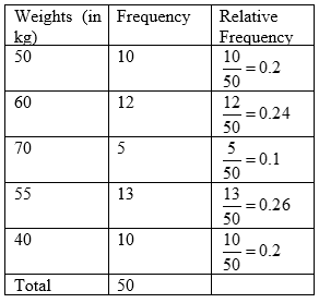
The frequency of a class divided by the total frequency is called the relative frequency of that particular class. The frequency distribution table showing the relative frequencies is called relative frequency distribution or relative frequency or percentage table. Relative frequencies are generally expressed as a percentage. The sum of the relative frequencies of all the classes is 1 or 100%.
Relative Cumulative Frequency Distribution
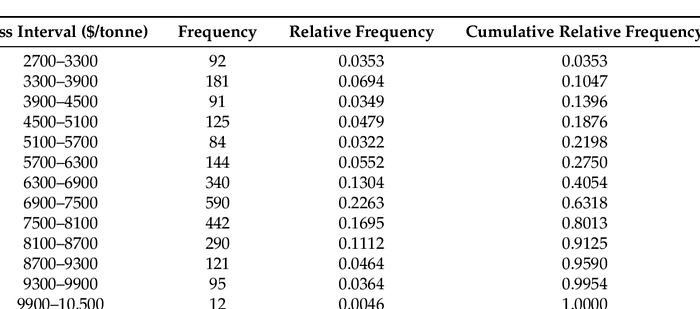
The cumulative frequency of a class divided by the total frequency is called relative cumulative frequency. It is also called percentage cumulative frequency since it is expressed in percentage. The table showing relative cumulative frequencies is called the relative cumulative frequency distribution or percentage cumulative frequency distribution
Bivariate Frequency Distributions
It is known that the frequency distribution of a single variable is called univariate distribution. When a data set consists of a large mass of observations, they may be summarized by using a two-way table. A two-way table is associated with two variables, say X and Y. For each variable, a number of classes can be defined keeping in view the same considerations as in the univariate case. When there are m classes for X and n classes for Y, there will be m × n cells in the two-way table. The classes of one variable may be arranged horizontally, and the classes of another variable may be arranged vertically in the two-way table. By going through the pairs of values of X and Y, we can find the frequency for each cell. The whole set of cell frequencies will then define a bivariate frequency distribution. In other words, a bivariate frequency distribution is the frequency distribution of two variables.
The following table shows the frequency distribution of two variables, namely, age and marks obtained by 50 students in an intelligent test. Classes defined for marks are arranged horizontally (rows) and the classes defined for age are arranged vertically (columns). Each cell shows the frequency of the corresponding row and column values. For instance, there are 5 students whose age fall in class 20–22 years and their marks lie in the group 30–40

Advantages & Disadvantages of a Frequency Table
1- Rapid Data Visualization (+)
2- Visualizing Relative Abundance (+)
3- Complex Data Sets May Need to be Classed Into Intervals (-)
4- Frequency Tables Can Obscure Skew and Kurtosis (-)
Finally, let’s sum up the entire process from scratch till creating a frequency table:
Question 1: How to find frequency distribution?
Answer: We can find frequency distribution by the following steps:
- First of all, calculate the range of the data set.
- Next, divide the range by the number of the group you want your data in and then round up.
- After that, use class width to create groups
- Finally, find the frequency for each group.
Question 2: Define frequency distribution in statistics?
Answer: In an overview, the frequency distribution of all distinct values in some variables and the number of times they occur. Meaning that it tells how frequencies are distributed overvalues in a frequency distribution. However, mostly we use frequency distributions to summarize categorical variables.
Question 4: Why are frequency distributions important?
Answer: It has great importance in statistics. Also, a well-structured frequency distribution makes possible a detailed analysis of the structure of the population with respect to given characteristics. Therefore, the groups into which the population breaks down can be determined.
Question 5: State the components of frequency distribution?
Answer: The various components of the frequency distribution are: Class interval, types of class interval, class boundaries, midpoint or class mark, width or size o class interval, class frequency, frequency density = class frequency/ class width, relative frequency = class frequency/ total frequency, etc.
